“If the maintenance costs get high enough, we will just replace it.” This phrase represents the prevailing attitude about asset management that is taught in graduate business schools and heard in conference rooms in most, if not all, manufacturing and production facilities around the globe.

From the perspective of reliability concepts, the phrase is a manifestation of a belief system that represents an inaccurate understanding of where high maintenance costs come from and what the proper method for reducing them would be.

From a financial perspective, the phrase is correct at face value, but the actual threshold limit for the replace decision point is substantially higher than what is commonly used in industry. Let’s take a deeper look at the logical pitfalls of the commonly held beliefs as well as an explanation of the calculation of the threshold limits for the replacement decision.

The Existing Paradigm

Though it has been proven wrong many times over since Nowlan and Heap produced their seminal work on reliability analysis in the 1960s, many asset managers still operate under the mistaken impression that older assets exhibit higher failure rates. This mental paradigm, while correct for approximately 11 percent of the failure modes for a sufficiently large group of assets, is inaccurate for the other 89 percent of the failure modes for that same group of assets.

There is a mountain of continually growing evidence that clearly demonstrates the majority of failure modes for any given asset are a function of how the machine is treated, and not a function of how old the asset is. Quite simply put, a well-treated asset will have a lower failure rate than an ill-treated asset, regardless of age. The treatment, in this context, speaks to how machines are operated, lubricated, cleaned, and maintained, as well as how the parts for those machines are designed, selected, transported, stored, and installed.

Further, financial managers have made capital monies more easily obtainable than additional budgetary monies, thereby allowing the ingression of maladaptive behaviours into the organisation. The behaviour these policies encourage is one of deferment instead of vigilance.

There is no doubt financial managers were not consciously encouraging these behavioural choices. Surely, the act of making budgetary monies more difficult to acquire was intended to force asset managers into a behavioural pattern of caring for their assets such that additional budgetary monies were not needed. However, making capital monies easier to obtain allowed for an unhealthy option of just buying a new one when the maintenance costs were too high.

As a result, many asset managers choose the easier route of buying a new asset rather than changing the behaviours of their personnel to force a higher grade of care for the assets. This is a financial mistake. This financial policy costs the organization even more money than the higher maintenance costs, as can be easily seen in life cycle cost (LCC) modelling.

The Hard, Cold Truth

Life cycle cost models are designed to help asset managers understand the entire cost of an asset rather than just the initial purchase price of an asset. The use of LCC models encourages the consideration of all aspects of the costs and benefits of selecting a given asset among multiple choices.

Well-defined models include both the costs and benefits of aspects such as design, manufacturing, acquisition, storage, installation, commissioning, operations, maintenance, decommissioning, removal, and disposal. Typically, LCC models are built within spreadsheets, and each of these aspects can have their own row or multiple rows to model those costs and benefits.

The models cover several years to completely model the life cycle of the aspect. Typical models range from 7 to 15 years, but can go up to 25, 30, or even 50 years depending on the estimated life cycle of the asset. Most model lengths are more dependent on technological obsolescence than on end-of-useful life estimations for the reasons noted in this article. These costs and benefits are then summed to a total for each time period, and then divided by a factor to account for the time-value of money.

The factor is often called the “hurdle rate” and represents the profit the organization could make using that same money in other ways. It should be noted that the hurdle rate for different alternatives can be different, depending on whether the alternative requires capital monies or not. The sum total of annual totals once the time-value of money has been accounted for is called the net present value (NPV), as the evaluation of future events needs to be performed in present day dollars.

It is the NPV upon which project alternatives are supposed to be evaluated, though most organizations manage themselves into a financial corner where they have to succumb to the most immediate needs of the moment in order to survive. These organizations do not make decisions on NPV as much as they make decisions on initial purchase price.

Making decisions on initial purchase price is an excellent way to ensure the organization will always be in that financial corner. To break out of that corner, start making decisions on the NPV of the LCC. The difference is usually more immediate and more impactful than most decision makers believe it will be.

The use of computer spreadsheets dramatically increases the usefulness of NPV calculations in LCC models with respect to asset management decisions. Asset managers can use some of the spreadsheet functions to easily analyse what-if scenarios and find the repair versus replace threshold limits quite easily.

Step 1: Create an LCC model for the replacement of the existing asset. We will call this model Option A: Buy New.

Step 2: Create an LCC model, in the same spreadsheet as Option A, for keeping the old asset. We will call this model Option B: Keep Old.

Step 3: Use the spreadsheet tools to vary the maintenance costs of Option B, until the NPV for Option B is equal to Option A.

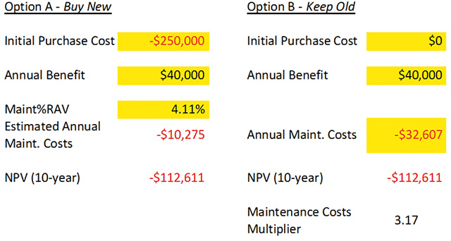
Step 4: Divide the annual (or total) maintenance costs for Option B by the annual (or total) maintenance costs for Option A. This is the Maintenance Costs Multiplier or the threshold limit for the repair versus replace decision. See Figure 1 as an example.

Figure 1. The organization would have to spend more than 3.17 times as much on maintenance for the old asset as they expect to spend on maintenance for the new asset.

In Figure 1, the organization would have to spend more than 3.17 times as much on maintenance for the old asset as they expect to spend on maintenance for the new asset to make the purchase of the new asset a sound financial decision.

Argument #1: The New Asset Will Be More Productive.

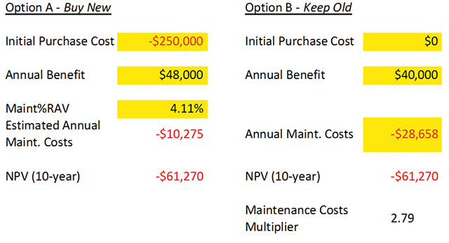
Even if the new asset is 20 percent more productive, the additional benefit does not offset the initial purchase price (see Figure 2). Further, to offset the effect of the initial purchase price in the scenario noted in Figure 2, using a maintenance cost for Option B that is twice that of Option A, the productivity of the new asset would have to be 61 percent more than the existing asset.

Figure 2. If the new asset is 20 percent more productive, the additional benefit does not offset the initial purchase price.

Rare is the case that the asset upstream can provide that much more input and the asset downstream can accept that much output. If that is the case, then it is a sound financial decision; if not, reconsideration is necessary.

Argument #2: Did Your Model Account for the Downtime Being Caused by the Old Asset?

No, downtime is not in the model, nor should it be in most instances. There are two reasons for this. Reason #1 is that with the inspection methods available today, the detectability of most machinery defects is over 95 percent. This degree of detectability means that the vast majority of machinery defects can be found and corrected long before emergency downtime is required.

Thus, downtime is more a function of the quality of your inspection program and the maturity of your asset management schema and not a function of the asset’s age or condition. Reason #2 is that very few systems suffer downtime from one and only one asset. Rare is the case for a system that does not have a backlog of work, and therefore decisions to schedule downtime are shared across multiple assets and not a single asset.

Argument #3: The Old One Will Require a Rebuild to Get It to a Maintainable Condition.

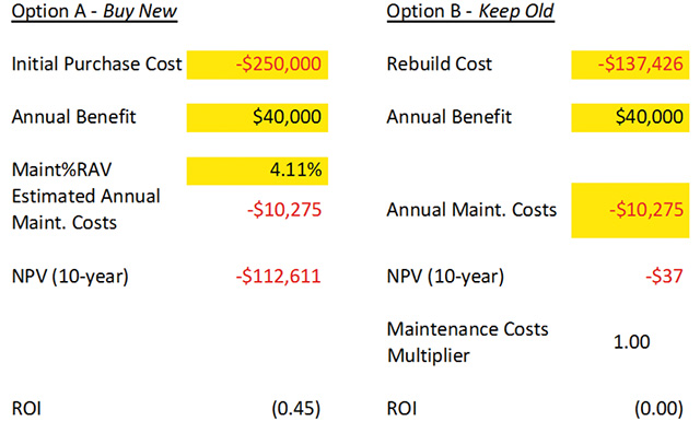
Many times, the conversation between the reliability engineer and the asset manager is around the cost of rebuilding the old asset versus the cost of buying a new one. The model in Figure 3 shows this precise scenario.

Figure 3. The cost of rebuilding the old asset versus the cost of buying a new one is shown here.

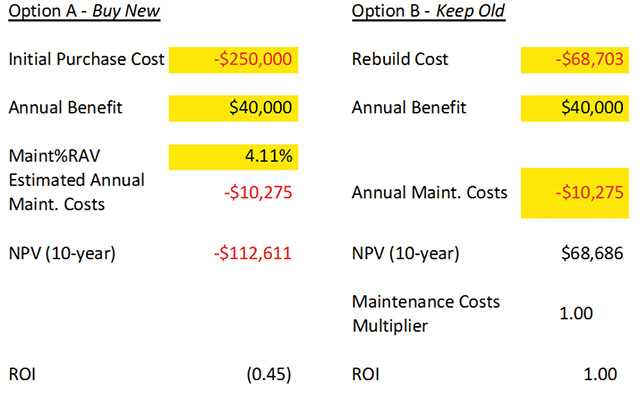
You can see that if the maintenance costs are expected to be the same, which is logical for a like-for-like replacement, for an ROI of 0.00 (breakeven) the rebuild costs of the old one can be as much as 55 percent of the costs of the purchase and installation costs of the new one. Setting an ROI of 1.00, then the rebuild costs can be only 27 percent of the costs of getting a new one (see Figure 4).

Figure 4. With an ROI 1.00 the rebuild costs can be only 27 percent of the costs of getting a new one.

Remember, these threshold limits will change as the initial purchase cost of the new system changes. To model each scenario correctly, the what-if scenario has to be run in your spreadsheet each time for each new value. There is no universally-accepted ROI for such calculations. The required ROI is dependent upon the financial manager and, of course, the financial climate at the time of the request.

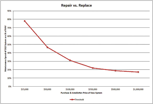
As the initial purchase cost of the asset changes, so do the threshold limits. Using the scenario in Figure 1, a set of tables and a graph can be created to represent the variation in threshold limits. See Figures 5 through 7. Note the lower right-hand value in the tables in Figures 5 through 7.

Figures 5-7. Using the scenario in Figure 1, a set of tables and a graph can be created to represent the variation in threshold limits.

Even with a $1M project and horrible maintenance costs, the threshold limit is still around 1.5. You can go out to $100M for the initial costs and down to maintenance cost of 25 percent of replacement asset value (RAV) and still the threshold limit will be 1.03.

Figure 8. The graph is for a analysis with no rebuild costs, just higher maintenance costs.

Figure 8 has the handy graph for a simple analysis with no rebuild costs, just higher maintenance costs. If the project is below the red line, keep the old one. If the calculation puts the project over the red line, buy the new one.

Implications of the New Paradigm

There are several implications of these threshold value calculations. Implication #1, in a repair versus replace scenario, there is virtually no practical maintenance cost for the old one where the purchase of a new one is a sound financial decision. Implication #2, where a high initial rebuild cost is concerned, the desired ROI determines the threshold limit for rebuild costs.

However, the most challenging implication, given what we now know about threshold limits, is that asset managers are always money ahead to keep the assets in a maintainable state, and not let them degrade to the point where a rebuild versus replace scenario has to be calculated. This implication is proven true in that we know there is no practical limit to maintenance costs that would be greater than overcoming the initial purchase prices of a new one.

This leads us to the final implication that is almost exclusively for financial managers; without calculating threshold limits, do not make capital monies more readily available than expense monies, as that policy drives financially unsound decisions. In short, this entire article is just one more piece of compelling evidence that it is always cheaper to keep the asset maintained than it is to allow it to degrade and then try to repair or replace it. n

Author Bio: Andy Page, Principal Consultant for Allied Reliability Group, has over 20 years in the maintenance and reliability field, helping organizations with unique and advanced maintenance system and organizational problems, from identification and analysis through successful solution deployment. He is well grounded in reliability and maintenance engineering topics, with particular emphasis on PdM technologies, continuous improvement processes, and education. Andy is a Certified Maintenance and Reliability Professional (CMRP) through the Society for Maintenance and Reliability Professionals (SMRP) as well as a Six Sigma Master Black Belt.

NOTE: This article appeared in the Dec 2015/Jan 2016 issue of Uptime magazine.

 

Andy Page

Principal Consultant, Allied Reliability Group, USA

pagea@alliedreliability.com